Click this link for Algorithm Example
Introduction
- Algorithm is a basic tool and is the first step of problem-solving that helps in getting the effective solution of a simple problem.
Definition
- An algorithm is a set of sequential step by step procedure, each of which has a clear-cut meaning and usually written in ordinary/natural English Language to solve a given problem in finite number of steps.
- An algorithm is defined as a complete, unambiguous, finite number of logical steps for solving a specific problem.
Characteristics/Properties
Every algorithm must satisfy the following criteria i.e., a typical algorithm has following characteristics –
(i) Input: An algorithm must take at least one or more well defined input values.
(ii) Output: An algorithm must provide at least one or more output values.
(iii) Definiteness : No instructions should be repeated i.e., each step of the algorithm must be precisely and unambiguously stated.
(iv) Finiteness : An algorithm must terminate in a finite number of steps.
(v) Effectiveness : An algorithm should be simple and focused on its main objectives. Each step-in algorithm must be effective.
(vi) Generality : The algorithm must be complete in itself so that it can be used to solve problems of a specific type for any input data.
Features
- No matter what the input values are, an algorithm terminates after executing a finite number of instructions.
-
It is a step-by-step instruction for solving a particular task in finite amount of time.
-
Algorithm is an effective method for solving a problem expressed as finite sequence of instructions.
- It may be possible to solve to problem in more than one way, resulting in more than one algorithm. The best choice of various algorithms depends on the factors like reliability, accuracy and easy to modify. The most important factor in the choice of algorithm is the time requirement to execute it, after writing code in High-level language with the help of a computer.
- The algorithm which will need the least time when executed is considered the best.
Advantages
- The algorithms are very easy to understand because it is step wise process.
- Algorithm is programming language independent.
- Algorithm makes the problem simple, clear, correct and effective.
- Every step in an algorithm has its own logical sequence so it is easy to debug.
- An algorithm acts as a blueprint of a program and helps during program development.
- It is easy and good practice to first develop an algorithm of a problem and then convert it into a respective flowchart and then into a computer program.
Disadvantages
- Algorithm is mostly effective for simple problems.
- Algorithms use text-based tools.
- Algorithms are time-consuming.
- Complex tasks are difficult to handle using algorithms.
- Difficult to show complex branching and looping in algorithms.
- Understanding complex logic through algorithms feels very difficult.
Rate of Growth/Classification of an Algorithm
- Growth rate is used to analyse the algorithm.
- The greater the amount of data, larger the number of resources required by an algorithm. Therefore, there is a resource growth rate for a piece of code in the form of function f(n).
- Commonly used rates of growth to analyse the algorithm are –
(i) Constant function algorithm:
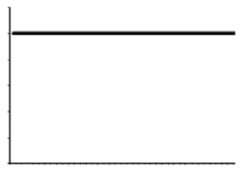
- A constant resource need is one where the resource need does not grow as the size of input data grow.
- It is the simplest function with some fixed constant c such as c = 1 or c = 5 etc.
-
The constant function is calculated as: –
- The constant function is used to add two numbers, initialising value to a variable, comparing two numbers.
- Here, the next instructions of most programs are executed once or at most only a few times. If all the instructions of a program have this property, we say that its running time is a constant.
- The graph of such growth rate is represented by a horizontal line.
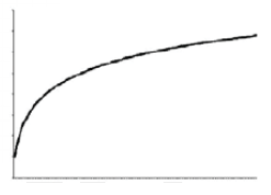
- Logarithmic growth rate is a growth rate where resource need increases by one unit each time the data is doubled.
- The logarithmic function is calculated as: –
f(n) = logb n for constant b > 1
- This function is defined as x= logb n if bx = n, where value b is called base of the logarithm (2 or 10).
- When the running time of a program is logarithmic, the program gets slightly slower as n grows.
- The running time commonly occurs in programs that solve a big problem by transforming it into a smaller problem, cutting the size by some constant fraction.
- When the value of n is a million, log n is a doubled whenever n doubles, log n increases by a constant, but log n does not double until n increases to n2.
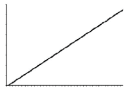
- The linear function calculated as:
- A linear growth rate of an algorithm is a growth rate where the resource needs and amount of data directly proportional to each other.
- The growth rate of linear function is represented by a horizontal line.
- When the running time of a program is linear, it is generally the case that a small amount of processing is done on each input element.
- This is the optimal situation for an algorithm that must process n inputs.
- The example of linear function includes comparing a number to each and every element of size n require n comparisons.
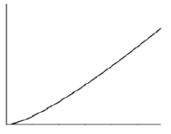
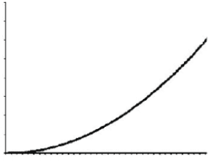
- This type of function is calculated as:
- The function that assigns to an input n, the value of n times the logarithm base-two of n.
- A log linear growth rate is slightly curved, i.e., for lower values than higher ones.
- The running time of this algorithm arises for algorithms but solve a problem by breaking it up into smaller sub-problems, solving them independently, and then combining the solutions.
- Here, when n doubles, the running time more than doubles.
- The example of log linear include possible algorithm for sorting n numbers.
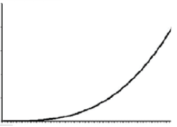
- The quadratic function is calculated as:
- The function assigns an input value n, the function f assigns the product of n with itself.
- When the running time of an algorithm is quadratic, it is practical for use only on relatively small problems.
- Quadratic running times typically arise in algorithms that process all pairs of data items (mostly n a double nested loop) whenever n doubles, the running time increases four-fold.
- The example of this algorithm includes nested loops, where inner loop implements linear number of instructions and outer loop implemented linear number of times.
- The cubic function is calculated as:
- This algorithm process triples of data items (mostly in a triple – nested loop) has a cubic running time and is practical for use only on small problems.
- Here, whenever n doubles, the running time increases eight-fold.
- The example includes Matrix Multiplication with three loops.
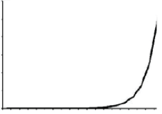
- The exponential growth rate is one where extra unit of data requires double number of resources.
- It is calculated as:
- This algorithm with exponential running time is likely to be appropriate for practical use.
- Such algorithms arise naturally as “brute–force” solutions to problems.
- In this algorithm, whenever n doubles, the running time squares.
NB:
The use of n above may be the number of data items to be processed or degree of polynomial or the size of the file to be sorted or searched or the number of nodes in a graph etc.
The most common computing order of complexity are –
O(1) > O(log2 n) > O(n) > O(n. log2 n) > O(n2) > O(n3) > O(2n) > n! > nn
![]()
0 Comments